Planetary Equilibrium Temperature Calculator

Equilibrium temperature is the temperature a planet or moon would settle at if it were a bare blackbody: it soaks up starlight, radiates that energy back to space as infrared, and carries no heat of its own and no atmosphere to trap warmth. When the world is in balance, the power it absorbs from its star exactly matches the power it sheds as thermal radiation, and that balance point fixes a single number in kelvins.
Astronomers reach for this number constantly because it strips a planet's thermal state down to the two things that matter most at first order: how much stellar energy arrives, and what fraction bounces straight back off. That makes Mercury, Earth, and a newly announced exoplanet directly comparable on the same footing. Feed the tool a stellar flux in W/m² at the planet's orbit and a Bond albedo, and it returns the zero-greenhouse, uniform-temperature equilibrium value.
Where the formula comes from
Plain-text formula: T = [((1 - albedo) * flux) / (redistributionFactor * sigma)]^(1/4).
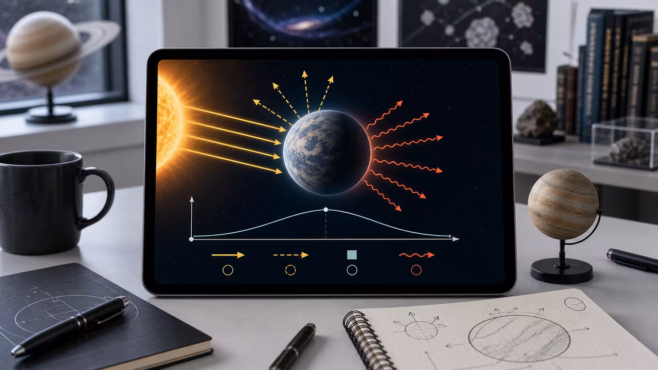
Everything rests on one steady-state accounting rule: energy in equals energy out. Absorb more than you emit and you warm up; emit more than you absorb and you cool. Left alone, a planet drifts toward the temperature where those two flows cancel. Two quantities set that point. The incident stellar flux F (W/m²) is the starlight power crossing a square meter at the planet's orbit — roughly 1361 W/m² at Earth, the value we call the solar constant. The Bond albedo A (0 to 1) is the share of all that incoming energy the world reflects; 0 is a perfect absorber, 1 a perfect mirror.
The outgoing side is governed by the Stefan–Boltzmann law, which ties a blackbody's emitted power per unit area to the fourth power of its temperature:
Here j is the emitted power per unit area (W/m²), T is temperature in kelvins, and σ is the Stefan–Boltzmann constant, about 5.670374419×10⁻⁸ W·m⁻²·K⁻⁴ (the CODATA 2018 exact SI value, last reviewed for this calculator on May 14, 2026). Now picture a sphere of radius R. It catches starlight only across its shadow — a disk of area πR² — but it glows from its entire surface, 4πR². The absorbed power is therefore (1 − A) F πR², while the emitted power is 4πR² σ T⁴. Setting them equal gives (1 − A) F πR² = 4πR² σ T⁴, and the πR² cancels off both sides. That single cancellation is why planet size never enters the answer: a boulder and a gas giant at the same flux and albedo run the same average temperature, even though the giant handles vastly more total energy.
Solving what remains for T leaves the standard result:
T = [ (1 − A) × F / (4 × σ) ]^(1/4)
Because temperature depends on the fourth root of absorbed flux, the model is stubborn: doubling the flux lifts the temperature by only about 19 percent. That fourth-root damping is exactly why planets do not swing wildly in temperature when their star or reflectivity changes modestly.
Choosing flux, albedo, and the redistribution factor
Two boxes drive the core result, plus one dropdown. Enter the stellar flux F as the starlight reaching the orbit — 1361 W/m² for Earth, higher for closer or brighter stars, lower for distant or dim ones. Enter the Bond albedo A between 0 and 1; useful anchors are about 0.30 for Earth, 0.12 for the Moon, and 0.75 for cloud-shrouded Venus, and a higher albedo always means a cooler world. The redistribution factor decides how the absorbed heat is spread before it radiates. Leave it at 4 for a rapidly rotating world that shares heat evenly over its whole sphere. Choose 2 to average over only the lit dayside, appropriate for a slowly spinning body, and 1 for the substellar point of a tidally locked planet that never turns its hot face away. The general form the tool evaluates is T = [((1 − A) × F) / (n × σ)]^(1/4), where n is that factor. The result appears in kelvins, with Celsius (subtract 273.15) and Fahrenheit shown alongside, though the physics itself lives in kelvins.
Reading the number you get back
Treat the output as a globally averaged baseline, not a forecast of what a thermometer on the ground would read. It shines as a reference point for comparing worlds, as a first sanity check on habitability once you layer in atmosphere and pressure, and as a knob for sensitivity studies — nudge the albedo up to mimic spreading ice and watch the balance cool. The gap between this baseline and reality can be enormous: Earth's equilibrium value sits near 255 K (−18 °C), yet the real global mean hovers around 288 K (15 °C) because our atmosphere holds back part of the outgoing infrared. As a rough guide, results well below 273 K point to a frozen surface without help from a greenhouse, values in the 250–300 K window are where liquid water becomes plausible under the right pressure and warming, and anything far above 300 K signals a scorched world in the mold of Mercury or Venus.
Working one case by hand makes the arithmetic concrete. Take Earth at F = 1361 W/m² and A ≈ 0.30. The absorbed flux is (1 − 0.30) × 1361 ≈ 952.7 W/m². Dividing by 4σ ≈ 2.2682×10⁻⁷ gives about 4.20×10⁹ K⁴, and the fourth root of that is roughly 255 K — the −18 °C baseline noted above, a stark reminder of how much greenhouse warming Earth actually enjoys. Swap in the Moon at the same 1361 W/m² but a darker A ≈ 0.12, and the absorbed flux climbs to about 1197.7 W/m²; the same steps land near 270 K (about −3 °C). The real lunar surface roasts and freezes far past that spread because it has no air and turns slowly, but its long-run average radiative balance tracks the simple estimate well.
The table below stretches that reasoning across a handful of worlds. The figures are illustrative — real conditions shift with atmospheres, rotation, internal heat, and more.
| Object / Scenario | Stellar Flux F (W/m²) | Bond Albedo A | Equilibrium Temperature (K) | Notes |
|---|---|---|---|---|
| Earth (idealized) | 1361 | 0.30 | ≈ 255 | Observed mean surface ≈ 288 K due to greenhouse effect |
| Moon | 1361 | 0.12 | ≈ 270 | Large day–night swings; little to no atmosphere |
| Venus (zero-greenhouse model) | ≈ 2613 | ≈ 0.75 | ≈ 230 | Actual mean surface ≈ 737 K because of extreme greenhouse |
| Mars (idealized) | ≈ 590 | ≈ 0.25 | ≈ 210 | Thin CO₂ atmosphere; real conditions somewhat warmer than bare rock |
| Hypothetical exoplanet in habitable zone | 1000 | 0.30 | ≈ 238 | Could reach Earth-like surface temperatures with moderate greenhouse effect |
Limitations the model deliberately accepts
The calculation earns its clarity by ignoring a great deal, and knowing what it ignores is the difference between using the number well and misreading it. It assumes no greenhouse effect, so the planet radiates straight to space as if any atmosphere were perfectly transparent to infrared — yet gases like CO₂, water vapor, and methane routinely push real surfaces well above the baseline. It assumes a single uniform temperature everywhere, when day and night, equator and pole, land and ocean can differ by tens or hundreds of degrees; the redistribution factor lets you lean toward or away from that assumption but never removes it. It treats the world as a perfect sphere radiating evenly in all directions, holds the Bond albedo constant even though clouds, seasons, and shifting ice change reflectivity, and ignores internal heat from radioactive decay, tides, or leftover formation warmth — a real omission for icy moons like Europa or for gas giants that glow with their own energy. Finally it presumes a settled radiative steady state, so sudden volcanism or a flickering star falls outside its reach. Read the output as a reference line to measure real climates against, and reach for atmospheric composition, pressure, circulation, and internal heat whenever you need the actual conditions on the ground.
Common questions about equilibrium temperature
Sources. The radiative balance is textbook physics; the constants and planetary reference values come from published data.
- Stefan–Boltzmann constant, 5.670374419×10⁻⁸ W·m−2·K−4, exact in the revised SI: NIST CODATA, Stefan-Boltzmann constant.
- Solar irradiance at 1 AU, Bond albedos and published equilibrium temperatures for the planets: NASA Goddard Space Flight Center, Planetary Fact Sheet.
- Nominal values for the astronomical unit and solar luminosity used by the orbit helper: International Astronomical Union resolutions on nominal solar and planetary conversion constants.
How is equilibrium temperature different from actual surface temperature?
Equilibrium temperature comes from a bare radiative balance with no greenhouse effect and a uniform surface. Real surface temperature answers to greenhouse gases, convection, the latent heat of water, oceans, clouds, and terrain, so observed means usually run warmer than the equilibrium value — by hundreds of kelvins in the extreme case of Venus.
Why does planetary radius drop out of the formula?
A planet intercepts starlight over its disk (πR²) but radiates from its full surface (4πR²). When you set absorption equal to emission, the πR² appears on both sides and cancels, leaving only flux and albedo. Bigger worlds move more total energy, yet their average temperature can match a pebble's at the same flux and albedo.
How does the greenhouse effect change things?
A greenhouse atmosphere lets visible starlight through to the surface but is partly opaque to the outgoing infrared, absorbing and re-emitting it and trapping some of the energy on the way out. That lifts the surface above the equilibrium value this tool reports, and the size of the gap is a rough gauge of how strong the greenhouse is.
Does it work for moons and dwarf planets?
Yes — the formula applies to any roughly spherical body in radiative balance, including moons, dwarf planets, asteroids, and artificial worlds, as long as you know the incident flux and Bond albedo. For a moon, use the flux arriving from the central star at that orbit, not the reflected glow from its parent planet.
What if I only know the orbital distance, not the flux?
Use the orbit helper below the main form. Flux falls off with the square of distance, so a star of luminosity L at distance d delivers F equal to L divided by four pi d squared. Entering the luminosity in multiples of the Sun and the distance in astronomical units scales the solar constant of 1361 watts per square metre directly, and the derived flux is written into the flux field for you.
Why is the redistribution factor 4 for most planets?
A planet intercepts starlight across its circular cross-section, an area of pi R squared, but radiates from its entire surface, an area of four pi R squared. The ratio of those areas is four, so a rapidly rotating planet that spreads absorbed heat evenly divides the incoming flux by four. Use 2 for a body that redistributes heat only across its dayside, and 1 for the substellar point of a tidally locked world with no heat transport at all.
Mini-Game: Albedo Balance
Use this optional game to build intuition before you run scenarios. Move the planet's reflectivity slider to keep the modeled equilibrium temperature near the target while stellar flux changes. Bright worlds reflect more incoming energy and cool down; darker worlds absorb more and heat up.
| Equilibrium temperature (K) | — |
|---|---|
| Equilibrium temperature (°C) | — |
| Equilibrium temperature (°F) | — |
| Absorbed flux (1 − A) F (W/m²) | — |
| Emitted flux per unit area σT⁴ (W/m²) | — |
| Relative to Earth's 254.6 K baseline | — |
| Greenhouse offset against the observed value | — |